Formula to get first second and third highest values

In this post I will show you how to look up the first, second, third and so on values. This formula can also be used to create Pareto charts which I will also go through in the next post.
In previous posts I touched on the idea of having a file that could quickly query different sheets depending on drop down lists that would be made up of a few of my post topics. This is the final part of that file and I’ll also cover how to put it together in a later post.
Formula To Get First, Second And Third Values
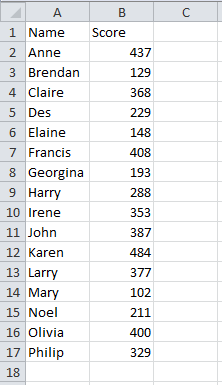
To demonstrate the formula to get the first, second, third and so on, values we will start with a list of names and scores as below.
In order to get the first, second, third and so on values, we need to identify them.
We will use the Rank function to rank the values.
Starting in C2, the Rank function is:
- =RANK( to start the function
- B2 is the number that you want to rank
- B:B is the ref that you want to rank your number against
- 0) is the order you want to sort by, 0 is descending and 1 is ascending. We want to sort in descending order,where the highest value is 1, second highest is 2 and so on.
The full formula for cell C2 is =RANK(B2,B:B,0). Copy this down for the remaining names/scores.
![]()
I have deliberately changed my values in B2 and B3 to be both 900. This is to demonstrate that if there are two numbers the same, they will be given the same rank.
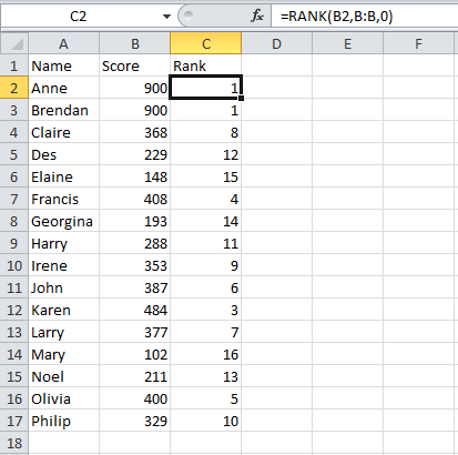
The scores in rows 2 and 3 are both ranked as 1. As you may already know, when using a lot of lookup functions, only one value will be retrieved, so if we looked up what was ranked as 1, the function would normally only return the first value ranked as 1 that it finds.
We are going to add a ‘helper column’ that will remove the chance of two scores having the same rank.
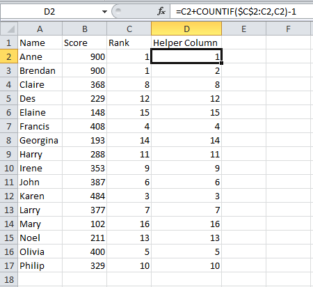
This helper column counts how many times a rank appears and removes duplicates.
Basically, the formula is taking a Rank, and adding it to how many times the rank has been used already and deducting 1.
Take the formula in D2, it is taking the rank in C2 (1), counting how many times that rank is used in the range C2 to C2 (1) and deducting 1. This results in 1+1-1=1.
Moving down to D3, it is taking the rank in D3 (1), counting how many times that rank is used in the range C2 to C3 (2) and deducting 1. This results in 1+2-1=2.
This has removed the chance of two values having the same rank.
The formula in D2 is:
- =C2 taking the rank in C2
- +COUNTIF($C$2:C2,C2) this counts how many times the value in cell C2 appears in the range C2 to C2 and adds it to the value of C2. Note the use of dollar signs in the first C2, this is because when you drag/copy the formula down you want the range to always be from C2, but you want the second part of the range to change to C3, C4 and so on.
- -1 deduct 1
Now that we have ranked our values and removed the chance of duplicate ranks, we can now get our first, second and third values.
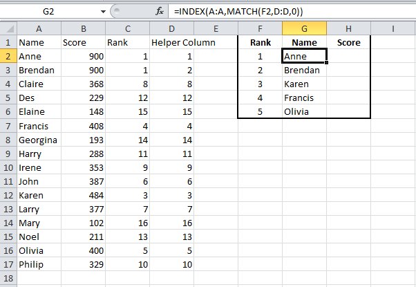
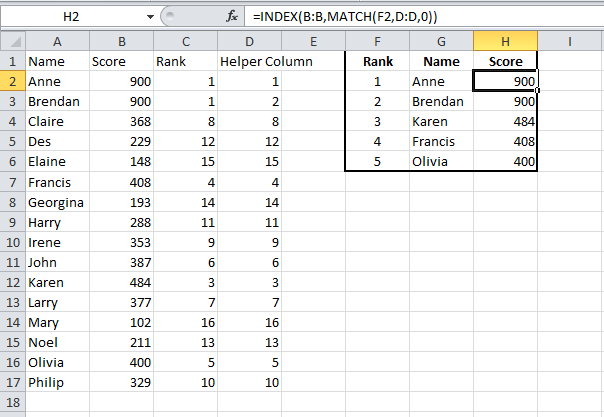
In column F2 to F6, I’ve listed the numbers 1 to 5 and we will retrieve the names and scores against the highest to fifth highest ranked name/score.
In column G I use index match to retrieve the name against the highest ranked name.
This post covers Index Match in more detail, the breakdown of the function for this example is:
- =INDEX( we start the INDEX function
- A:A we want to retrieve the name from column A
- MATCH( we are going to start a MATCH function to get the row_num for our INDEX function
- (F2,D:D,O)) our lookup value will be 1 (from cell F2) and we are going to look for this value in column D. We use 0 to indicate that we want an exact match.
The above function will look up the rank 1 from F2 in column D and retrieve the name from column A against that rank.
Copy the formula down for the remaining values 2 to 5.
Use the same function and amend to retrieve the scores from column B.
That covers the first part of this topic, showing you how to retrieve the first, second, third and so on, values. If you wanted to retrieve the lowest, second lowest and so on, values then you could have changed the order of your RANK function to be ascending.
The next post will show you how to use the above to create a Pareto chart.