FORMULA TO GET LAST ROW NUMBER

In Excel, you can write a formula to get the last row number containing data.
At first, it’s not an obvious formula, but using Excel’s own logic and lookup function can give you the answer.
When i was first asked by somebody for a formula to get the last row number I almost immediately saw a few other places that I could use this formula myself.
There are relatively simple VBA instructions that can get the last row number for you, but some of the files that I work on cannot be macro enabled, so I have to use formula instead.
This post along with some others will be used together to create a data validation drop down list that can be used to reference different sheets depending on the values of the drop down lists.
Since each component of that tool has it’s own uses, I will write separate posts about each part.
For now, we will concentrate on the formula to get the last row number.
Formula To Get Last Row Number
A lookup function will be used in our formula.
The final formula will be made up as follows:

Doesn’t make much sense does it?
Let’s talk through the logic of it….
Data
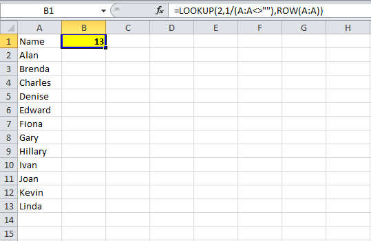
To demonstrate, I’ve added some names to cells A2 to A13 – this could be text or numeric, it doesn’t matter.
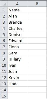
As you can see, row 13 is our last row and should be the answer from our formula at the end.
Logic Test
In column B I will add a logic test, again, this is purely for demonstration and to explain the formula.
This test is going to check if the corresponding cell in column A is blank or not.
For cell B2, the formula is =A2<>””, this means is A2 not equal to blank?
I will also copy this formula down to row 16, so we can see the result for blank cells.
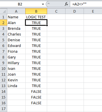
As you can see for B2 to B13, the result of the logic test is “TRUE”, the value in column A is not equal to blank.
For B14 to B16 the value is equal to blank, so our logic test is FALSE.
In column C, we will divide 1 by the result of the logic test.

Numerically, TRUE equates to 1 and FALSE equates to 0.
Dividing 1 by TRUE gives us 1 (1/1=1) and dividing 1 by FALSE returns the #DIV/0! error because we are trying to divide 1 by zero.
Lookup
In cell D2 I enter a simple LOOKUP function.
This is going to lookup “2” in column C.
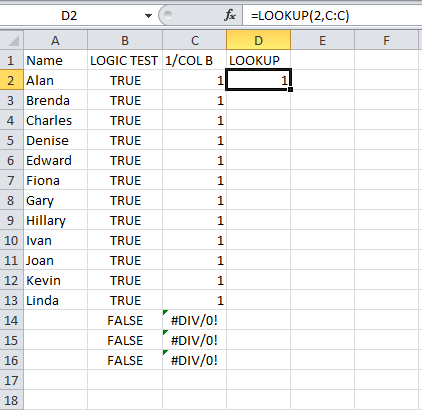
As you can see, there is no 2 in column C, so the LOOKUP returns the closest number it can find, which is 1.
It is not obvious at this point, but the 1 that the LOOKUP has found is the last 1 in column C, this is in cell C13.
Final Formula To Get Last Row Number
We are going to use a LOOKUP function now and apply what we have learned so far.
If you use the Function helper, you want to use the “lookup_value, lookup_vector, result_vector” function.
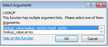
The first part of our formula (lookup_value) will be 2.
This will be similar to the LOOKUP in cell D2 earlier. We know that 2 won’t appear in our lookup_vector but we want to find the last 1.
Our lookup_vector will be similar to column C and B from earlier in this post.
Instead of testing if A1 is equal to blank, then A2 and so on, we will test all of column A as an array.
The second part of our formula will be 1/(A:A<>””).
We will search for 2 in the logic test of column A and it will not find 2, but it will then go to the last 1 it finds, which as you can see from our logic tests is the last row, 13.
Row
So far our lookup will return the value 1, it searches for 2, can’t find it so it retrieves the next lowest number it finds.
The last part of our formula will give us the row number of the last 1 the formula finds in column A, this is ROW(A:A).
What we have entered so far in columns B and C was purely for demonstration and to explain the formula to get the last row number.
You can delete them.
Before doing so, note that each individual formula refers to one cell (A1, A2, A3, A4 and so on).
If you look at the syntax for the final formula in the image above you will see the curly brackets {}, this means the range is being treated as an array, but when creating the formula we don’t have to create the formula as an array formula.
In B1, I have entered the final formula, and you can see the result is 13, the row number of the last row in column A containing data.
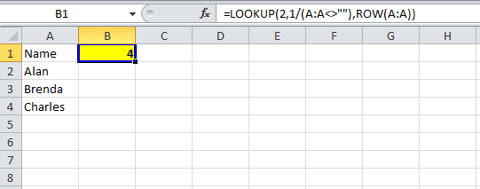
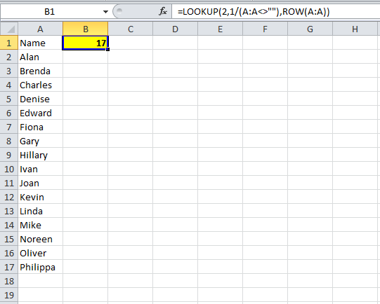
As you can see below, when I delete rows or add rows to column A, this formula will give the last row number.
This lookup formula gives you the last row of a given column containing data.
In a future post post I will go through how to retrieve the 1st, 2nd, 3rd, etc. highest values using LARGE, INDEX and MATCH functions.
I have already covered the INDIRECT function in an earlier post, combining these I will show you how to put this altogether to retrieve the top 5 values from various sheets depending on drop down list values.