SUMIF
The SUMIF formula is a really useful formula for adding the values in cells based on set criteria.
This post will build on what you have seen already in the IF Statements post and will use the example of game scores.
To demonstrate this, we will use an example of a list of scores each player achieves.
The table below is on a sheet called “SCORES” and lists the scores each person achieved.
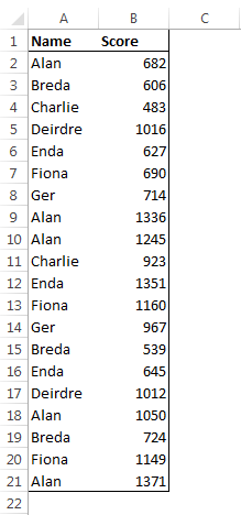
As you can see some players have played more than one game. There is a second sheet called “SUMMARY” and in this sheet there is a table with each person’s name and a field for total score.

We are going to use a SUMIF formula to look up each person’s name in the “SCORES” sheet and add up their scores to give each person’s total scores. Note, if a VLOOKUP was used here it would only return one score for each person and not a total score.
The SUMIF formula can be broken down as SUMIF(range, criteria, sum_range).
Our first formula will be =SUMIF(Scores!A:A,A2,Scores!B:B). This formula is entered in cell B2 of the “SUMMARY” sheet.
Let’s walkthrough the formula
- =SUMIF( : This is a SUMIF formula and the paramaters will be contained within the brackets
- Scores!A:A : Our range is column A of the SCORES sheet. The range is where we are going to look for our criteria.
- A2 : Our criteria is in cell A2 of our SUMMARY sheet – note the sheet name isn’t needed here because the formula is being entered in the same sheet.
- Scores!B:B : The sum_range is the range to be added up if we find our criteria. In our case, the scores that we want to sum are in column B of the SCORES sheet.
In short, we want our formula to look for our name (criteria) in column A of the SCORES sheet (range) and if it finds our criteria, to add up the values in column B of the SCORES sheet (sum_range).
A simple SUMIF formula can look long and complicated like =SUMIF(‘C:\Users\JayTray\Documents\sitework\[some other file.xlsx]Sheet1′!$B$1:$B$30,A1,’C:\Users\JayTray\Documents\sitework\[some other file.xlsx]Sheet1’!$AM$1:$AM$30).
Does this formula look anymore complicated than our first example? If you have read and understand the previous post on brackets and commas you should be able to break it down.
The SUMIF formula is SUMIF(range, criteria, sum_range). Our second formula is made up this same way and is no different, but it looks longer. Let’s breakdown this formula into its 3 components.
- ‘C:\Users\JayTray\Documents\sitework\[some other file.xlsx]Sheet1’!$B$1:$B$30 : Our range that we are going to look for our criteria is between cells B1 and B30 of “Sheet1” of a file called “some other file.xlsx” which is saved in a folder called “sitework” in my documents folder on my C drive. This whole section brings us up to our first comma, so we know that it is the address of our range and is just a filepath address, name, sheet and cell reference. If this file was open at the time then we don’t see the filepath, we would see the filename, sheet name and cell range. If the range was in our same file but a different sheet, then we would only see the sheet name and cell range. If the range was in the same sheet as our formula then we would only see the cell range.
- A1 : Our criteria is in cell A1 of our sheet. If the criteria was in a different sheet, or file then you would see the sheet name and or file name/path similar to what you have seen in the range explaination.
- ‘C:\Users\JayTray\Documents\sitework\[some other file.xlsx]Sheet1’!$AM$1:$AM$30 : Similar to the explanation of our range, the sum_range is between cells AM1 and AM30
Use the commas to breakdown the formula into it’s 3 main components and you shouldn’t get too lost!
Remember….. where are you searching?, what are you searching for? and what are you adding up?.
