Excel VBA Macros : Your First Formula
The Story So Far…
If you have been following this string of posts, you will have created a macro which has so far changed headings in a file and also formatted them.
This is a link to the last post.
At the end of the last post I also asked you to make some changes to the macro yourself, compare your code to this…
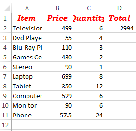
In the last post I said that for this post we will create our first formula through VBA, by selecting cell D2 and multiplying the price in B2 by the quantity in C2.
Our First Formula
Multiplication Through VBA
Open the file you have created so far, or download a copy of the file as it should be from here Macros_Example_C
Press Alt and F11 to see the code created so far.
At the end of our macro (but before the “End Sub” line) we will start creating our first formula.
Code Snippet – Multiplying 2 Cells
Range(“D2”).Select
ActiveCell.FormulaR1C1 = “=RC[-2]*RC[-1]”
The first thing we need to do is make D2 the active cell, so we select it.
Then with D2 as the active cell we want to change the value of the cell to our formula.
Note the two equals symbols! If you were to manually type this formula in Excel you would start with an equals sign, it is no different here, we put an equals sign into our formula after the double apostrophes.
I use the relative references for R (rows) and C(columns) in relation to the active cell.
In this case, we are in cell D2, multiplying B2 by C2, so they are both on the same row. We do not have to enter a numeric value beside R in our formula, we can leave it as R.
We are going to change the column values though, column B is 2 columns to the left of D, so the relative number here is “-2”. Column C is one column back from D, so the relative number here is “-1”.
So, we are going to multiply the cell on the same row, two columns back (RC[-2] = B2) by the cell on the same row, one column back (RC[-1] = C2).
That is it! Simple as that!
Coding formulas through VBA is different to normal formulas when you first look at them. I find the relative references easy to follow, if I have a large file with alot of rows and columns then I might record a small macro performing the formula and check that code against my code to make sure I’m right.
There are other ways to do this same type of formula, but this is the one I use, feel free to Google and find your own preferences if you want.
What Next?
At the minute we have started formatting headers, and put a formula in column D2.
Why is the formula only in D2?
I could tell you how to copy the formula down to cell D11 right now, but what happens the next time this report is run and it goes down to cell D15 or D12,345? Your macro will only copy the formula down to D11.
Next time we will create our first variable which will find out the last row of data, and then use that to copy our formula. Before that though, I will share a post about moving around Excel with the arrow keys and Ctrl and Shift keys.


