0

Excels Scenario Manager

This post looks at Excel’s Scenario Manager function in 4 main sections.

1. Setting up scenarios with the Scenario Manager
2. Switching between scenarios
3. Creating a summary report comparing scenarios
4. Overcome one of the downfalls of scenario reports – making sense of “changing cells”

If you are familiar with the scenario manager summary reports already but want to know how to change the “changing cells” description to make more sense then you can skip to section 4.

If you are new to scenario managers, don’t worry we are going to start with the basics.

Section 1

Setting up scenarios with the Scenario Manager

We are going to use the example of estimating costs for next year based on percentage increases.

• Column A lists the cost descriptions
• Column  B shows this year’s costs for each cost type
• Column C shows the expected percentage increase next year
• Column D contains a formula that calculates next year’s estimate costs based on the % increase

 

You can find the Scenario Manager on the DATA ribbon.

Click on “What-If Analysis” and then select “Scenario Manager”.

This opens the Scenario Manager dialog box.

Initially, there are no scenarios to show.

We are going to add our first Scenario.

• Click “Add…”

• Give the scenario a name.  For the first one, I’m calling this “Most Likely”
• For “Changing cells” I want to change the percentage values between cells C2 and C5, so I select this field and then highlight those cells.
• Click the “OK” button

• The values for each of the changing cells are all at 0.1 (10%) which is what is already in each of the cells.  I am going to leave these values at 0.1 for now.
• Click the “OK” button

• You can now see that you have 1 scenario created.  Create a second one by clicking “Add…”
• Repeat the steps above again but with the following changes:
  • Scenario Name = “Worst Case”
  • All values to be changed to 20% (0.2)
• Add a third scenario as follows:
  • Scenario Name = “Best Case”
  • All values to be changed to 5% (0.05)
• Add a fourth scenario as follows:
  • Scenario Name = “Pay Increase”
  • The value for C3 to be changed to 25% (0.25) and all other values left at 10% (0.1)

 

• You can close the Scenario Manager box by clicking the “Close” button
• You can reopen it again by selecting Scenario Manager from the DATA ribbon again
• You can edit any of the scenarios by selecting it and clicking the “Edit…” button.

In the next section we will see the results of some of our scenarios.

 

Section 2

Switching between scenarios

• With the Scenario Manager dialog box open, select one of the scenarios listed (Pay Increase for example)
• Click the “Show” button
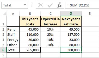
• The data in our file changes from this:

• To this:

The staff amount has changed and all others are 10%.

Show the other scenarios and watch the percentage amounts change, and they in turn change the estimate values for next year.

This has so far allowed us to see one scenario at a time.

In the next section we will use the scenario manager summary function to compare all scenarios.

 

Section 3

Creating a summary report comparing scenarios

Creating a summary report is surprisingly easy.

• If it is not already open, open the Scenario Manager dialog box
• Click the “Summary…” button

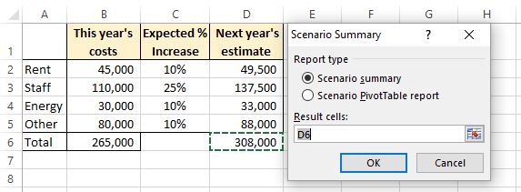
• Select the Scenario summary as your report type
• The result cells is D6 – this is the cell(s) with the formulas that are impacted by your various scenarios.  In our case, the total estimate costs for next year will be our result cell.
• Click the “OK” button

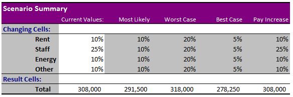
In the scenario summary, you can see the percentage changes for each cell we change.

Below each list of percentages you can also see the result cells values, so for each scenario we created, this is the total value of costs for next year.

One of the downfalls of the scenario summary is that the changing cells and result cells refers to the cells (C2, C3, D6, etc.) and these are not very descriptive.

The next section shows you how to change these to be more descriptive.

 

Section 4

Making sense of “changing cells”

The easiest way to change this is to name your cells.

• Click on the first cell to be named – C2
• Above the column headers and to the left of the formula bar you can see “C2” in the Name Box.  This shows the cells that you are currently in.

• Change the value in C2 to “Rent” and click return
• Repeat for cells C3, C4 and C5, changing the name to match the cost description
• Repeat for cell D6, naming it “Total”

 

Now, if you run the summary report again, you will get the reference to the names you gave cells, rather than the standard cell reference.

This makes more sense and you can see quicker what each cost line is, rather than having to refer back to your original worksheet to see what C2, for example, referred to.

 

I would recommend going through these steps again.

Create your own scenarios, give them names, create your own summary reports, change the result cells, etc. to see what results you get.

The Scenario Manager is a very useful tool, sometimes it is overlooked or thought of as being more complicated than it actually is – as you can see (hopefully) it is actually relatively straightforward once you have tried it a couple of times.