Paste Special
Paste Special is another time saving trick that may be going underused.
You are probably already familiar with the cut, copy and paste functions in a lot of applications.
- Copy allows you to make a copy of selected or highlighted data to be pasted somewhere else
- Cut allows you to remove selected or highlighted data and then paste it somewhere else
- When you cut or copy, something is added to your clipboard, pasting allows you to take something from your clipboard and place it where you want.
So, what is different about Paste Special?
Paste Special gives you more options and control over what you paste from your clipboard, and what you do with it.
Different applications can offer you different options when pasting.
In the cases below I will be using Paste Special in Excel, and I will not be covering all options, but hopefully you will see enough to feel comfortable with trying them yourself.
The options I use most often are highlighted below.

To demonstrate examples, I will use the table in the section below, and different versions of it:
Paste Special Formula
Column B of the file gives the line number of the table.
1 is entered in the first line (obvious enough).
The second line adds 1 to the line above it and we want to copy this formula to all the lines below it, so we get 2;3;4;5;6;7;8;etc.

By simply copying and pasting the formula, Excel will copy the formula but also the formatting of the cell being copied.
In our case, we are copying cell B3 which has no border, so when we copy it down it overwrites any borders we had set.

However, if we copy B3 and then highlight the relevant rows and go to Paste Special and select “Formulas”, Excel will copy and paste the formula only – it will not paste any formatting or borders from the original cell.

Paste Special Values
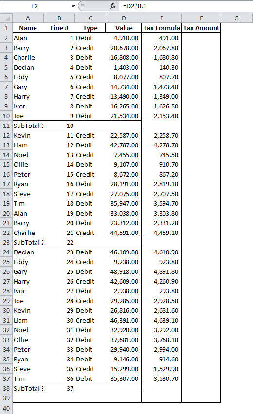
To demonstrate Paste Special Values, I have added a formula to column E.
This just multiplies the value in column D by 0.1 (or 10%).
We are going to copy column E to column F
When we copy column E and paste to F the formula is changed to multiply the values in column E by 0.1, which as you may have noticed is not what we want.
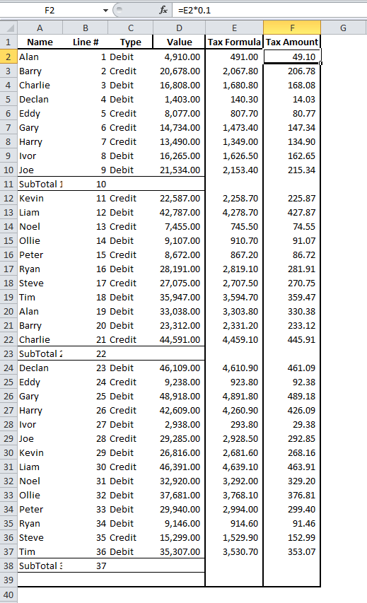
If we only wanted to paste the value, then use Paste Special and select “Values”. Excel takes the value (the result of the formula) and pastes it in column F.

Paste Special Comments
Another way to use Paste Special would be to copy comments on a cell to others.
I have added a comment to cell A2 and want to copy this comment to all other cells in that column – pasting the comment would obviously be faster than creating the comment for each person.

If we copy cell A2, which includes the comment, and paste it to all others in the column we would get:

Excel has pasted the value, formatting, borders and comments of A2, but we only want to paste the comments.
Copying A2 and then selecting “Comments” from the Paste Special list would give us this:

Only the comments have been copied and pasted. The values, formats, borders, etc were not pasted too.
Paste Special Multiply
Paste Special also allows you to perform certain operation. One that I use quite often is the multiply option.
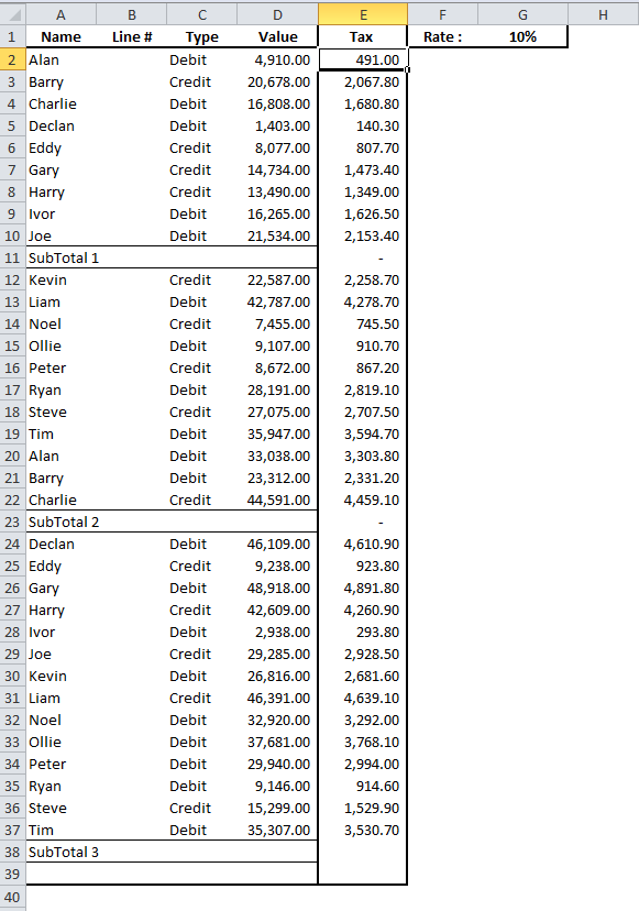
Column E contains the same value as D, but I want to multiply this by the 10% rate in G1.

To do this, I copy the 10% in G1 and then highlight the numbers in column E and select “Multiply” from the Paste Special options.
This then multiplies the 10% that we copied by each of the values we applied the Paste Special operation to.
You’re probably wondering why would you ever need to use this? I use this option on a weekly basis to convert a batch of numbers to negative numbers. There is more on this at the bottom of this post.
Paste Special Transpose
Transpose allows you to convert a horizontal list to a vertical list, or vice versa.
Below is a horizontal list of all our names.

By copying the above list and then in A3, I select “Transpose” from the Paste Special options.
My horizontal list is transposed to a vertical list.

Converting a Batch Of Numbers To Negatives
An example of where a batch of numbers may need to be converted to negatives would be in the case of a downloaded bank statement for example.
Assuming that you want all the credit numbers to be negatives, it is possible to simply type a dash (-) before the value.
But if you have a large number of numbers to change, this can be boring and time consuming, plus there is a chance that you may miss numbers to be changed.

Personally, when I have to complete this task I:
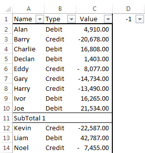
- Filter for credits
- Copy “-1” which is typed somewhere to the side
- Highlight the filtered results and Go To visible cells
- Paste Special multiply – which will multiply the credits by -1, giving a negative number.
Note : The following may seem like a lot of steps and a long way to complete the task, but it is quick to do when you get used to it.
Step By Step…
- Filter column B for “credit”
- In cell D1 (or anywhere to the side) type in “-1”

- Copy the -1
- Highlight the row of numbers in column C
- Open the Go To dialog box by pressing Ctrl and G together

- Press the “Special” button
- Select “Visible cells only”
- Press “OK”

- Now Right-click on one of the highlighted numbers and from the Paste Special menu, select “Multiply”
- Clear your filter and admire your handiwork.
Remember when you are using the “Multiply” operation of Paste Special, you are also selecting to paste “All” from the top section of the Paste Special unless you change it from the default “All”.
So, why did we go through all those “Go To” steps? If you didn’t, the Paste Special may apply to all numbers in the highlighted range, even if the filter has them hidden.
By using Go To “Visible cells only”, you are only selecting what the filter has not hidden and won’t affect any hidden values.
[grwebform url=”http://app.getresponse.com/view_webform.js?wid=4307503&u=CucD” css=”on”/]
