A Quicker Way To Create VLookUps Across Multiple Columns
Recently I have been asked by a few people for a quicker way to create VLookUps across multiple columns.
In each case the user wanted a VLookUp to pull in several columns of data, but did not want to have to create a VLookUp for each column (one case would have been over 20 columns of data).

I have covered VLookUps in an earlier post, if you are not familiar with them click here to read the earlier post.
For demonstration purposes I have created a file with two sheets, one with sales details and one with details of parts.
![]()
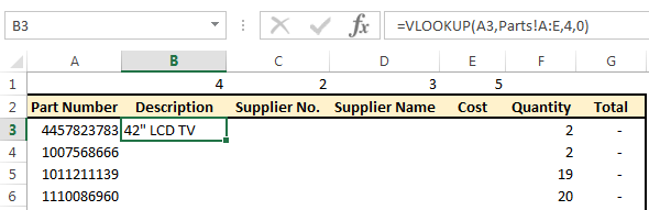
The “Sales” sheet contains a list of part numbers sold and their quantities. Column G contains a formula multiplying the quantity in Column F by the cost that will be in Column E.
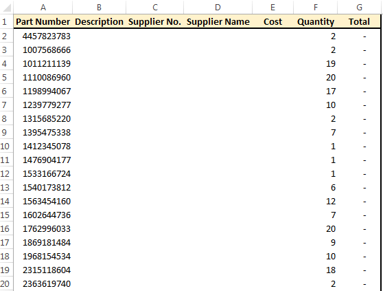
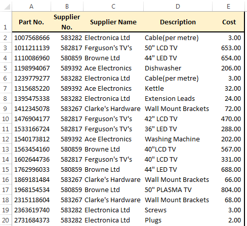
We will fill in the details for Columns B to E from the “Parts” sheet (extract below).
Normally the VLookUps in columns B and C would look like this:
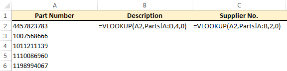
A VLookUp would be created for each column and dragged down for all relevant rows.
This is OK if you have just a few rows of columns to look up, but the users that came to me had a lot more (1 case had about 5 columns relating to addresses alone plus more for fax numbers, phone numbers, contact names, email addresses, etc). He did not want to have to create a lot of individual VLookUps across all the relevant files he was working on.
I showed these users a quicker way to create VLookUps across multiple columns with just a small change to a standard VLookUp.
Step 1 – Column Index Numbers
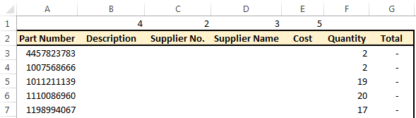
The first thing I did was add a row at the top that will be hidden later.
Above each column that I will be entering a VLookUp in, I have entered the column index number that I would be using in the VLookUps for that column. So, for example, the column index of the “Description” column is 4, so I entered 4 above the “Description” column. These numbers will be used in our VLookUps in a minute.
Step 2 – First VLookUp
Next, I create my first VLookUp.
For the Table Array, I select the whole table, not just up to the column I am looking up.
Step 3 – Make LookUp Value Column Absolute
So far our VLookUp is no different to any other VLookUP, except the whole table has been selected.
Next, we want to make our look-up value absolute.
As we drag our formula to the right, “A3” becomes “C3”, then “D3” and so on.
By putting a dollar sign ($) in front of the column reference (A) we tell Excel that as we drag the formula to the right we want the look-up value to remain as A.
If we drag the formula down rows the row number will change from 3 to 4 to 5 and so on. We have only made the column reference absolute, the row number can still change which is what we want.
Our formula is now =VLOOKUP($A3,Parts!A:E,4,0).
Step 4 – Make Table Array Absolute
We have changed the look up value to “$A3” so that A does not change. On the table array, we want the A to stay the same as well. It doesn’t matter if the E changes or not, it won’t effect the results of our formula.
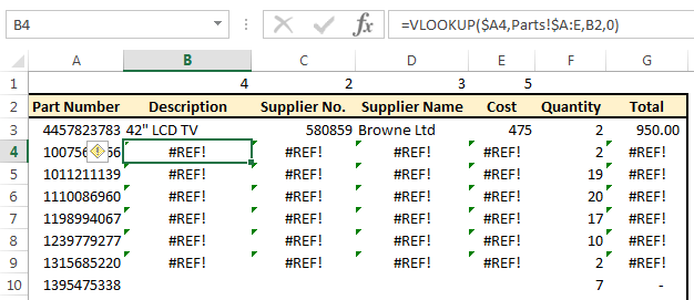
Our formula is now =VLOOKUP($A3,Parts!$A:E,4,0).
Step 5 – Update Column Index Number
If we dragged our formula as it stands across all columns we would get the description in every column because the formula is looking up column index 4.
We need to update the column index for each column we are entering a VLookUp formula in.
This is where we entered the column index numbers in row 1.
Delete the column index number (4) from the formula and replace it by clicking on the number entered earlier (in my case in B1).
If you drag your formula now across the columns you will see that it works, but if you drag it down a few rows you will notice a problem.
As we drag the formula across columns, the column index reference goes from B3 to C3 to D3 and so on, which is what we want.
But as we drag the formula down rows the row number of the column index section changes – which we don’t want.
By putting a dollar sign in front of the row number of this section (B$1) we tell Excel not to change the row reference, but to change the column reference as we drag this formula across and down.
This formula is now ready to be dragged across and down our entire table.

After hiding row 1, our table looks like this:
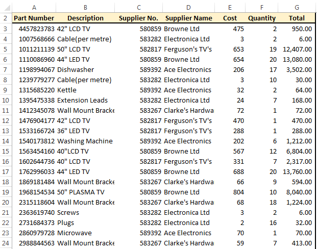
In the actual file that I have been using to demonstrate this, there are about 150 rows of data below the above rows.
Create VLookUps Across Multiple Columns
This may seem like a long post, but really the task of creating VLookUps across multiple columns involves one normal VLookUp, slightly amended and a hidden row of data to help speed up the process.
I have 4 columns that the VLookUp has been copied across in my example above, but in reality I have applied this technique to over 30 columns of data,so as you can imagine this technique has saved me (and now others) quite a bit of time.
Try it yourself, you might follow this post step by step, but very quickly it should become second nature changing a normal formula to suit your needs.
[grwebform url=”http://app.getresponse.com/view_webform.js?wid=4307503&u=CucD” css=”on”/]
