Data Validation List To Automatically Update Source Range
The last 2 posts looked at some Data Validation options in Excel for either a short list or a set range of cells.
This time we will use a formula in our Data Validation rule that will work out what range of cells to base the list on.
Data Validation Rule To Update As List Changes
In the image below, I have a range of data from cells C2 to C4, but I think I may end up adding to this list in the future.
So if I set the source of my Data Validation rule to be from C2 to C201, this allows me to add an addition 197 items to my list without having to change my Data Validation rule.

Makes sense right?
Unfortunately this can lead to a pain in the mouse-hand in the future.
When you do this you may end up with a lot of blank rows in your drop-down list and your list starts from the bottom. In the image below, I show how the drop down list looks without scrolling.
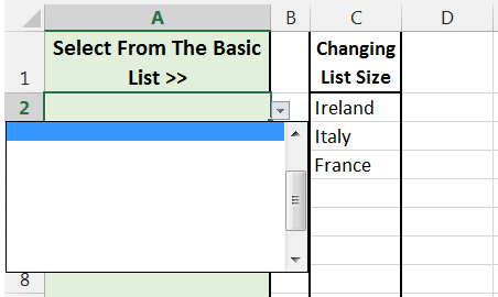
If you have to scroll through these blank values enough times you will find it very irritating.
Is there a way around this?
Yes there is, we will use a formula in our Data Validation source field that will work out the cell range we need. If we add to this cell range the formula will automatically update to allow for these additional cells.
Data Validation & Offset & CountA
The formula we are going to use is Offset and it’s function arguments are below.

The description for the Offset function is “Returns a reference to a range that is a given number of rows and columns from a given reference”.
Within the Offset function we will also use the CountA function.
The CountA function counts the number of non-blank cells in a range. We will use it to count how many cells in a column are not blank.
As the list in this column change, the result of the CountA function changes and so to does the Offset function.
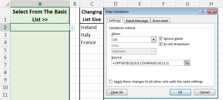
The final Data Validation rule is as below, I will now go through the formulas and how they go together.
Set up the Data Validation the same as you have done in the last 2 posts.
The source is now going to be:
- =OFFSET( – We are going to use an Offset function to determine our source
- $C$2 – Our list will start in cell C2. This is an absolute reference so put a $ before the C and 2. Or if you use your mouse to select the cell, Excel might do this for you.
- ,0,0, – Our number of rows and columns will be zero. Note the commas between each argument, this is very important throughout the full function.
- COUNTA(C:C)-1 – We are going to use the CountA function to calculate the height of our list (number of rows basically). The height will be the number of non blank cells in column C minus 1 (because we are going to ignore the header in cell C1)
- ,1) – The width of our Offset function is going to be 1, just 1 column wide. We are basing our Data Validation on column C only in my case, so just one column wide. We close off our function with a closing bracket.

Now if I add to the list in column C, without amending the Data Validation rule, you can see that my list automatically updates for the new values.

