Data Validation List Based On Range Of Cells

In the last post we created a short Data Validation List where we typed in the options for our drop-down list.
This time we will create a Data Validation List based on a list in a range of cells.

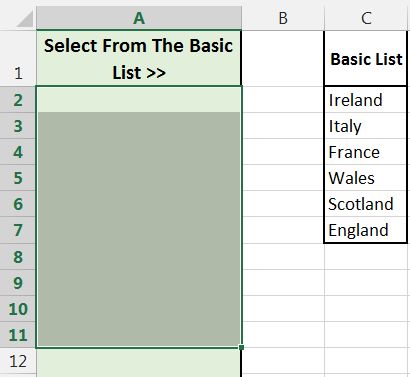
In this example we will create Data Validation Lists to column A and the options in our list will be based on the cell range C2 to C7.
My basic list is in column C purely for demonstration purposes, in reality your list does not have to be beside where you are applying the Data Validation Lists.
Data Validation List – Based on Range of Cells
- Select the cells that you want to apply the Data Validation List to. in my example cells A2 to A11.
- On the “Data” ribbon, select “Data Validation” from the “Data Validation” options.

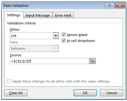
- Make the following changes:
- Allow: Select “List” from the menu
- Source: Select the range containing your list, in my case from cell C2 down to C7
- Click “OK”
Congratulations!!
You have created another Data Validation List in Excel.
The Next List
In the next post, we will look at creating a Data Validation List that can change its length to match the list you are basing your data validation on.
This is a fairly common issue with Data Validation Lists. You set up your validation rule based on cell C2 to C7 and then 3 more items are added, you need to update your list rules to now use C2 to C10 as the source.
The next list will change the source range to match the size of your list using the OFFSET function to help you.
