Create A Planner In Excel
It’s that time of year again when I start receiving requests for help with creating planners for the new year.
These planners are usually for teams or groups to organise holiday schedules and rosters.
This year I created a reusable planner that can be used in future years and also includes most of the features that different people ask me for.
Features Of The Planner
- The day for January 1st is selected from a drop-down list
- The remaining days are updated using formula
- Conditional Formatting is used to highlight the weekends
In the above image, Thursday was selected as the starting day. Below is an example of how it would look if Saturday was selected for the first day.
Below are the steps involved in creating a planner like this.
You can make whatever changes you want – for example, in the column to the right of the month, you might want to list the employee or team member names.
Planner Heading Layout
- From C3 across to AG3, the numbers 1 to 31 are listed
- From B4 down to Bx merge cells and change the text alignment (here Bx means down as many rows as you want for each month)
- Place a bottom border from C4 to AG4
- Put borders around the month’s section to suit your needs
- Copy the month (rows 4 to 9 in my case below) and paste it below the current month
- Repeat for each month of the year
- Shade out any dates that are not in a month (eg 29th to 31st for February)
First Day Of Planner
- Click on the cell relating to January 1st (C3 in my case)
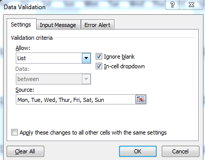
- Go to Data Validation on the Data ribbon
- In the “Settings” tab, change “Allow” to List
- Type in each day of the week, separated by commas under “Source”
- Click OK
- You can test this has worked by using the drop down list now available in this cell
Days Of The Week For The Planner
A Formula will be used to go to the next week day based on the previous day.
- In the cell for January 2nd (D4 in my case) enter the formula below
=IF(C4=”Mon”,”Tue”,IF(C4=”Tue”,”Wed”,IF(C4=”Wed”,”Thur”,IF(C4=”Thur”,”Fri”,IF(C4=”Fri”,”Sat”,IF(C4=”Sat”,”Sun”,”Mon”))))))
- Copy this formula across for the rest of January.
- For February 2nd, have the formula reference the 31st of January instead of the prior day.
- Repeat this for each month, the first day of the month should be based on the last day of the prior month.
Conditional Formatting For The Planner
There are two rule set up for each line in each month
- The first looks at the day of the week and if it is Sunday (“Sun”) then it highlights all rows for that day with a grey fill
- The second is similar but loos if the day is Saturday (“Sat”) and highlights all rows with the same fill
Reusing The Planner
This particular planner can be used as a template and reused from year to year.
The only exception, obviously being leap years, where there is an extra day.
Hopefully though, you understand enough of how this planner is put together to amend that yourself!
[grwebform url=”http://app.getresponse.com/view_webform.js?wid=4307503&u=CucD” css=”on”/]


