Excel Pivot Tables
In Excel, Pivot Tables are a quick and easy way to summarize, analyse and present data. The speed that the tables can be put together and rearranged makes them an invaluable and important tool for analysis and decision making.
The more data you have to analyse, the more obvious the uses of Pivot Tables are.
I have created a file with 500 rows of data that we will analyse using Pivot Tables.
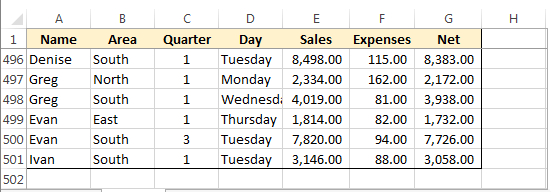
We have 7 columns of data in our example
- Name – let’s assume that this is made up of sales reps’ names.
- Area – the region or country is being split up into areas
- Quarter – the year is split into four quarters with 1 representing January to March
- Day – the day of the week between Monday and Friday
- Sales – the value of sales made on the day
- Expenses – the expenses submitted by the sales rep that day
- Net – the difference between sales value and expenses submitted each day.
What makes up the above data is not important, I just came up with these for the sake of demonstration.
We will create an initial Pivot Table and then review the data in different ways.
Create A Pivot Table
Before continuing – make sure that every column has a heading – Pivot Tables do not like blank headings.
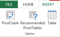
On the “Insert” tab of your Excel ribbon, you should see the first option as “Pivot Table”.
Select this and you will be shown a “Create Pivot Table” dialog box.
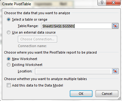
The top section of the box relates to the data to be analysed, this could be the table or cell range on your current file, or you can analyse data on another (external) file. In the majority of cases you might find that you are analyzing data in your current file. Excel will probably already have your data range selected.
The bottom part of the table relates to where you want the Pivot Table report to be placed, you can have it put on a new worksheet, or somewhere on an existing worksheet.
So far this may seem too easy to be true, but the truth is that Pivot Tables are that straightforward to create.
After you have selected your data source and where the data is to be placed, you will see a blank Pivot Table and also Pivot Table fields and options.

Let’s start analyzing our data.
Who made the most sales?
If we want to know who made the most sales then drag the “Name” from the list of fields to add to report and drop it under the “Rows” section.
Drag the “Sales” from the list of fields and drop it in the “Values” section.
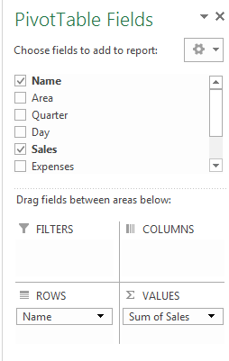
Our Pivot Table now shows us the total (sum) of sales for each rep.

Where did we make the most sales?
To analyse the sales data by area, drag the “Area” from the list of available fields down to the Row section and remove the “Name” from the Row section

Our Pivot Table then looks like this

What quarter did we make the most sales in?
To get the total of sales by quarter, remove Area from the Row section and drag down “Quarter”.


Further Analysis – Sales by person in each area
So far we have done simple analysis, who had the most sales, when did we have the most sales, where did we have the most sales.
Let’s take it a bit further and analyse who had sales in each area.
Set your Pivot Table fields as follows:
- Row = Name
- Column = Area
- Values = Sales
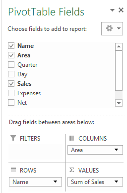
Our Pivot Table lists the names down the rows and the column headers going across are now the areas.

Further Analysis – Sales by person in each area for each quarter
Are you seeing how easy it is to change and analyse data? Let’s add a third element to our analysis.
We have seen an analysis of sales by person in each area, now let’s look at sales by person for each quarter in each area.
You can drag the “Quarter” from the available list of fields and drop it below the Name in the Row section.


Changing the order
We can change our Pivot Table to analyse sales by quarter broken down by person. To do this, just change the order in the Pivot Table options section
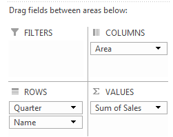
This then updates our Pivot Table as follows

Beside each quarter we see the total value and below each quarter we see the name of each person and their sales for that quarter for each area.
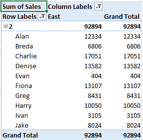
Filtering
Taking our above table, we can filter to only show the details for quarter 2 by filtering for 2 only.
This is the same as standard filtering in Excel, the filter is to the right of “Row Labels”.

We can filter further to see the sales for the East region only, by filtering “Column Labels”
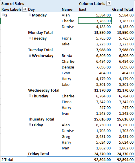
Even Further Analysis
We can add even more analysis to our table by adding “Day” to our Row section

Tabular Form
We can change the layout of the above Pivot Table, my personal preference is to use the “Tabular Form” layout
Right-click on the first Row field (2 in the case above) and select “Field Settings”.
On the “Layout & Print” tab, select “Show item labels in tabular form”.

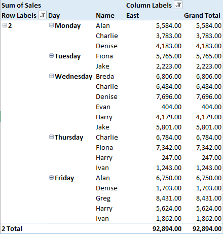
This changes our table layout, I have also set the Day Rows to be in tabular form too.

Number Formats
We will now change the number formats to use the 1,000 separator and 2 decimal places.
Click on any of the sales values and right-click and select Number Format.

Then set the number format as you want it.
Subtotal
At the minute each day of the week is subtotalled and also each area. To remove the subtotal of the days, right-click on a day and untick “Subtotal Day”
To put the subtotal back, again right-click and click “Subtotal Day”.
If it was a different Row we were working on, the option would be Subtotal and then the row name.
Summarize values by…
So far all the Pivot Tables have been the sum of the row and column data.
I have reset our table to just have the Name as the Row and Sales as the Value.
We have the total sales for each person.
Right-click on any of the sales values and go to “Summarize Values By”, another menu slides out and you are given options that you can summarize your data by, first pick “Average”.

This gives the average of each person’s sales.
Summarize the values by “Count” and you will see how many sales each person got.

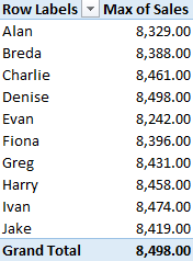
Summarize the values by “Max” and you will see what the highest day’s sales were for each person.
Try It Yourself
As with most Excel functions and tools, the best way to see how they work or what they can do is to try them yourself. If you don’t have a file you could practice on yourself, you could use this one pivot tables.
Quick, Easy & Flexible
I’m hoping that you can see how easily and quickly you can put together a variety of analyses and reports by simply dragging and dropping fields.
Pivot Table vs. Subtotals
For simpler analyses, Subtotal functions can be used to analyse data to a certain extent.
However, in my opinion, the options offered by Pivot Tables far outweigh those offered by Subtotals.
- With Pivot Tables the data does not have to be sorted first
- It is faster and easier to change the analysis options and fields on Pivot Tables
- The Pivot Table field table gives a clearer visual showing the make up of the Pivot Table
- The biggest benefit with Pivot Tables I find is the speed of them – each month I work on a file with over 20,000 rows of data and over 15 columns. Running the Subtotals I need on this file takes an average of about 40 minutes. The Pivot Table is completed within 2 minutes.
[grwebform url=”http://app.getresponse.com/view_webform.js?wid=2766903&u=CucD” css=”on”/]
