VLOOKUP
The VLOOKUP is one of Excel’s most useful functions. In its most common form, it is a database function which works with lists of things in databases, or Excel worksheets. Your list of things can be pretty much anything, names and phone numbers, part numbers and details, details of your album collections, etc.
A VLOOKUP retrieves information from a list based on a given unique identifier.
What does this mean? If we used a VLOOKUP to find the description for a part number that we supply, the formula will only return one result. If the part number is in our list more than once with different descriptions we will not get all these descriptions.
The identifier that we give the formula will have to be unique.
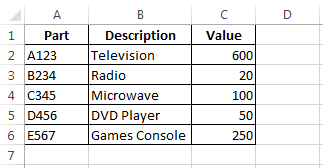
For demonstration purposes, we will use the Sales Department of an electrical retailer as an example. We have a database of items we sell, their descriptions, part numbers and values.
Obviously this is a rather small database and in the real world it would be much bigger.
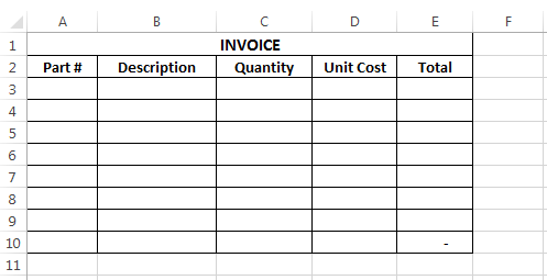
We have a template for an invoice. Every time we make a sale, we do not want to have to enter the full details each time. Instead we can enter the part number and the VLOOKUP will pull in the rest of the details.
Some things to note : Our database table is on the Parts worksheet and the range is from A1 to C6. The table we want to retrieve information from does not have to be in the same file, it can be another file.
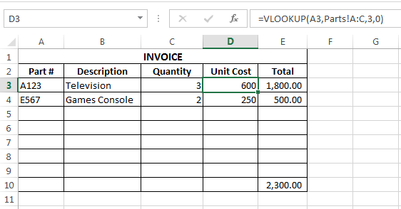
We will create an invoice for 3 televisions (part A123) and 2 games consoles (E567).
NOTE
Before continuing, if you have not already done so, or are not fully familiar with brackets and commas in Excel, I would advise reading this post on brackets and commas in Excel.
VLOOKUP
The VLOOKUP formula can be broken down as :
- What we want to look up
- The table we want to look in
- The column number the information is in
- The word FALSE (or number zero, which is the same)
Enter our two part numbers in A3 and A4 and the quantities in C3 and C4.

Starting our formula in Cell B3, our first formula is
=VLOOKUP(A3,Parts!A:C,2,0)

The formula syntax is VLOOKUP(LOOKUP_VAULE, TABLE_ARRAY, COL_INDEX_NUMBER, RANGE_LOOKUP)
Our formula can be broken down as follows
- lookup_value – A3 – this is what we want to look up, the part number in cell A3
- table_array – Parts!A:C – the table we are going to look up is columns A to C of the Parts sheet
- col_index_number – 2 – the result that we want to retrieve is in the second column of our table, which is the description
- range_lookup – 0 – entering zero, or the word ‘false’ here are similar. We are telling Excel that we want to find an exact match for our lookup_value only.
We can copy the formula down our ‘Description’ column of our Invoice – this will automatically populate the part description after we enter the part number in column A.
In D3, we are going to enter a similar formula, this time our column index number will be 3 which will retrieve the price of our parts.
The formula in column E simply multiplies our unit cost by quantity to give a sub-total, and cell E10 sums the sub-totals.
The Table Array
The value you are looking up must be the in the leftmost column of the table array you set. For example, in our case above if instead of looking up a part number, we wanted to look up a description that was entered, then the first column of our table array must be column B of the parts sheet.
The Table Array & Column Index Number
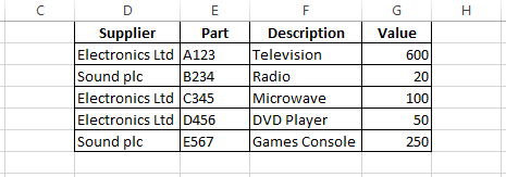
The table array does not have to begin in column A, it can begin anywhere, and it does not even have to be the start of our table – the lookup_value just has to be in the leftmost column of the array that we select.
The table below begins in column D, our part number, though is in column E, so our table array here will be from column D across to the right.
To The Right
The VLOOKUP works from the left to the right in the table array. If we wanted to look up a description and retrieve the part number then our database will not work because the part numbers are to the right of the descriptions. To correct this we could move the part numbers to the right of the descriptions.
Confused??
The VLOOKUP formula is often misunderstood. If you don’t get it at first don’t worry. Come up with your own tables and make it more meaningful to you. This formula is usually better understood and explained in a live classroom environment than reading it online.
#N/A
Are you satisfied that you have entered the formula correctly, but getting #N/A messages instead of what you would expect? This means that the value you are looking up is not available.
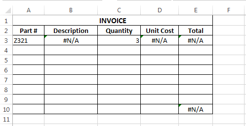
In our previous example we will delete the part numbers in A3 and A4 and create a new part number that isn’t in our parts list.
If you are happy that your formula is correct and don’t know why you are getting an #N/A, sometimes the quickest way to check this is note the part number and then go to the table array and find the part number. If the part is in the array, check the format of the look up value and the value in the table array. If it is just numbers, you may notice a small green triangle in the upper left hand corner of a cell.

In the above screen-extract, both cells have the number 12345. However, the top number is considered to be text by Excel even though there are no letters. You can see this because of the small triangle in the upper left corner of the cell. So if we were looking up a number (like the bottom number above) against a table that contained the same number, but as text format, Excel will not consider them to be the same and you will receive a #N/A error.
This is the most common reason I see for VLOOKUPs failing for people. Especially where numbers are concerned. This can be got around by changing the format of either the look up value or the table array to match each other.
You can either change them through Text-To-Columns or by using the message box that appears when you highlight cells with messages….

There are other ways to avoid #N/A by using IFERROR or IFISNA – these will be covered in future blog posts.
Reading The Formula
Sometimes a VLOOKUP formula can look daunting because they can get long. This next example is slightly longer than our previous formula.
=VLOOKUP(A3,[PARTSLIST.xlsx]Parts!$E:$G,2,0)
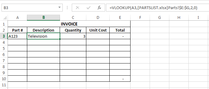
However, it is the same as our previous example, it is still giving us:
- What we want to look up
- The table we want to look in
- The column number the information is in
The difference here is that our table array is on the Parts sheet of a file called “PARTSLIST.xlsx” and this file is currently open. If the file was closed, we would also see the file path of the file with our table array, and it would be as follows:
=VLOOKUP(A3,’C:\Users\JayTray\Documents\BlogPostMaterial\[PARTSLIST.xlsx]Parts’!$E:$G,2,0)
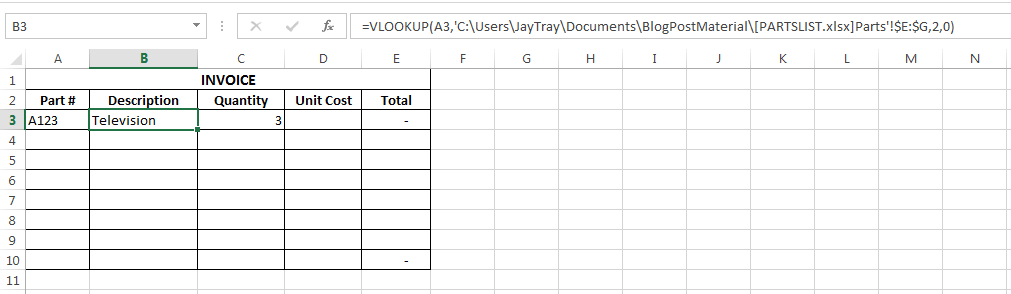
The VLOOKUP is longer and at first may seem more daunting, but if you pay attention to the commas, you will see that the second part of our syntax, the table array is made up of a file path, file name, sheet name and cell range.
Using The Formula Wizard
Another way to enter the VLOOKUP formula, or any formula is by using the wizard. To the left of the formula bar you can see “fx” clicking this opens the “Insert Function” wizard

If you select VLOOKUP from this you get a wizard box to complete the formula

You can enter each part of the formula in these boxes. To select cells or ranges, you can click the box to the right of each input box. The dialog box also gives you help as you move to each part of the syntax.
Why don’t I just show people how to use this?
I do show people how to use this wizard, but only after they are relatively comfortable with typing the formula themselves – in my experience, this will help them to understand formula created by others and to troubleshoot formula problems easier by being more familiar with the formula.
Other formula can be used within the VLOOKUP formula to complete parts of our syntax, but as I said before (many times!) pay attention to the commas and you can breakdown any of these formulas, no matter how long and complicated they look.
